Design and Analysis for Studies of Individual Responses Will G Hopkins Sportscience 22, 39-51, 2018 (sportsci.org/2018/studyir.htm)
|
|||||
Prescription
and monitoring of treatments Units for the dependent variable. Individual
responses as a standard deviation Individual
responses as proportions of responders Individual
responses as individual probabilities of responders. Statistical
models for simple designs Statistical
models for complex designs Update 9 Oct 2019. Link to slideshow on individual differences and responses presented at Hong Kong Baptist University in
October 2019. The reference
for the consensus statement referred to below as "in preparation"
is Ross R, Goodpaster BH, Koch LG, Sarzynski MA, Kohrt WM, Johannsen NM,
Skinner JS, Castro A, Irving BA, Noland RC, Sparks LM, Spielmann G, Day AG,
Pitsch W, Hopkins WG, Bouchard C. (2019). Precision exercise medicine:
understanding exercise response variability. British Journal of Sports
Medicine 53, 1141-1153. Assessment of individual responses to
interventions is an important issue, especially as ever cheaper genotyping
and pervasive monitoring provide researchers with subject characteristics
that could permit personalized targeting of training and other treatments to
improve health or performance (Hopkins, 2015; Hopkins, 2018a). In 2017 I took part in a
symposium on research aimed at quantifying individual differences in the
fitness response to changes in habitual physical activity. My contributions
on design and analysis were too extensive to include in more than summary
form in the consensus document arising from the symposium (in preparation).
Programs I wrote following the symposium in the language of the Statistical
Analysis System (SAS) for the analysis of individual responses are available here (Hopkins, 2018a), along with my deliberations on sample size for studies of
individual responses (Hopkins, 2018b). In this article I present the
full version of my approach to design and analysis of such studies. Research DesignsSimple designsIndividual responses are usually conceptualized in terms of differences between individuals in the changes (e.g., in fitness) that occur following a treatment (e.g., an increase in habitual physical activity). Implicit in such a concept is a pre-test and a post-test, separated by the period of the treatment, and the individual post-pre change scores represent the individual responses to the treatment. Changes due to error of measurement occur between two tests in every individual even in the absence of any treatment, so accounting for such changes requires a group of similar individuals who receive a placebo, inactive, or reference treatment. The changes that these control individuals experience can then be compared with those in the experimental group. The resulting design is a controlled trial, with the focus not just on the comparison of the mean changes in the two groups but also on the spread of the changes arising from the experimental treatment. This spread can be summarized as a standard deviation, as I will show later, but sample sizes required to estimate its magnitude with adequate precision are usually impractically large (Hopkins, 2018b). On the other hand, subject characteristics that could account for individual responses should be measured and included in the analysis as moderators or modifiers of the treatment effect, as their effects can often be characterized adequately with realistic sample sizes (Hopkins, 2018b). When effects of such subject characteristics are clear and substantial, they allow identification of the kind of individuals likely to be positive, trivial, or negative responders to the intervention. Such modifiers also provide evidence of individual responses and responders in the simplest of all designs, when there is an experimental group and no control group. It is possible to eliminate the pre-test in a controlled trial and analyze only post-test scores, which will themselves show more differences (a larger between-subject standard deviation) in the experimental group than those in the control group, when there are individual responses to the treatment. Such a "post-only" controlled trial may have more ecological validity than the usual pre-post design, because it involves the least interaction of researchers with their subjects. Unfortunately, sample size is always greater–and usually much greater–than in a pre-post design. Sample size in a post-only controlled trial reduces to the smallest of all designs when the same subjects experience the experimental and control treatments. These studies should be conducted as crossovers, in which the subjects receive each of the two or more treatments in a balanced order, with a sufficient washout period between treatments to allow subjects to return to their usual state. Crossovers are not a practical option for training studies, because the washout might not be complete even after many weeks or months, but they are the preferred design for estimating the mean effect of treatments that have only acute effects. Subject characteristics can also be included in the analysis to account for individual responses in a crossover, with one important exception: the baseline (control or pre-test) value of the dependent variable, the effect of which is confounded by regression to the mean. Estimation of the effect of this potential modifier requires either a repeat administration of the control treatment in the balanced sequence of treatments, or a design in which the crossover is conducted as a pre-post controlled trial, with the same subjects assessed pre and post each treatment. Certain aspects of design of a controlled trial need to be addressed to reduce the risk of bias of the mean treatment effect. The Cochrane handbook for systematic reviews of interventions provides details (Higgins and Green, 2011). Briefly, it is important for the study sample to be representative of the population subgroup of interest, ideally by stratified random sampling from the subgroup. Such sampling is usually impractical in controlled trials, and researchers instead should endeavor to select volunteers either reasonably representative for characteristics that could modify the effect of the treatment (e.g., level of habitual physical activity, body composition, age, sex) or with restriction to a sub-group that is homogeneous for one or more characteristics. Researchers should then avoid systematic differences between the experimental and control groups in the following: baseline characteristics (by random assignment, stratified or balanced for potential modifiers, including the baseline value of the dependent variable and known or suspected genotypic modifiers); exposure to factors other than the intervention of interest (by proscribing and monitoring for changes in behaviors that could affect the dependent variable); determination of the outcome (by administering assessments in the same manner to the treatment groups); and withdrawals from the study (by frequent interaction with subjects, by offering inducements for successful completion of any onerous training or testing regimes in the experimental group, and by offering the experimental program to control subjects, if they complete the control treatment). Prescription and monitoring of physical activity are also particularly important issues for reducing bias in training studies and are dealt with separately below. These aspects of design apply equally to reducing bias in the estimation of individual responses, but the possibility of bias arising from differences in error of measurement between the groups also needs to be addressed, as discussed below. Complex designsIn simple pre-post or post-only designs, assessment of the standard deviation representing individual responses is based on the assumption that the error of measurement is the same in the control and experimental groups. Pre-test errors of measurement are not expected to differ between groups, if the subjects are randomized or assigned in a balanced fashion to the groups. This expectation may not apply to error of measurement in the post-test, if the active or control treatments result in different habituation of performance or other dependent variable. Any differences in the change in error not accounted for in an appropriate analysis will confound estimation of the standard deviation representing individual responses; for example, a smaller error in the experimental group or a larger error in the control group will reduce the apparent magnitude of any individual responses to the experimental treatment. The solution to this problem is a repeat of the post-test with a period between the tests sufficiently short to assume any change in the individual response of each subject is negligible. The extra measurements allow separate estimation of the individual responses and the errors. An additional pre-test is not necessary but improves precision of estimation of all effects, including the individual responses. In designs for assessing adaptation or de-adaption to a treatment, there are two or more post-tests with sufficient time between tests for the possibility of changes to occur in the mean response and in individual responses. If the error of measurement does not differ between groups in the post-tests, the design requires only a single test at each post time point. If the error could differ, a repeat of the test after a short interval is required at each post time point, at the cost of increased participant burden and drop-outs. Sample-size estimationI provide an explanation first for the estimation of sample size for assessing the mean effect of the treatment. Sample size for assessing the magnitude of the standard deviation representing individual responses and for assessing subject characteristics that could explain the individual responses are then expressed as multiples of the sample size for assessing the mean. Sample size for the mean effect in a simple controlled trial or crossover can be estimated with freely available software, such as G*power (Faul et al., 2007). A spreadsheet is also available at Sportscience (Hopkins, 2006a). For pre-post designs, the user has to input a value for the error of measurement expected over the time between tests, because sample size is proportional to the square of the error of measurement. This error is often not available as such in publications, but an approximate value can be derived from similar studies of the effect, as shown in the Sportscience spreadsheet. There should also be provision for inputting the usual between-subject standard deviation, because inclusion of the pre-test value of the dependent variable as a modifying covariate reduces the sample size, depending on the relative magnitudes of this standard deviation and the error of measurement. Individual responses effectively increase the error of measurement and therefore the sample size, but it may be difficult to estimate the magnitude of the individual responses before the study is performed. In any case, to the extent that there are substantial individual responses, there will probably also be a substantial mean change due to the treatment, and sample sizes can be smaller for larger true effects. Therefore ignoring the effect of individual responses on the estimate of sample size is justifiable. Sample-size estimation also requires input of a value for the smallest important effect, the least clinically important change in the dependent variable. For fitness and other health-related indices, the best estimate would be the change associated with the smallest substantial change in risk of morbidity or mortality, a hazard ratio of 10/9 (Hopkins et al., 2009a). In the absence of such an "anchor-based" smallest change, standardization provides a "distribution-based" default: 0.2 of the between-subject standard deviation is widely regarded as the smallest important value for assessing differences or changes in means of continuous variables. Thresholds for moderate, large, very large and extremely large changes are given by 0.6, 1.2, 2.0 and 4.0 of the between-subject standard deviation and can be used to provide a more nuanced assessment of the mean change (Hopkins et al., 2009b). The final requirement for sample-size estimation is maximum acceptable rates of Type-I (false-positive) and Type-II (false-negative) errors, the defaults for which are 5% and 20% in null-hypothesis testing. In the approach to inference based on acceptable uncertainty in magnitude of effects (Hopkins and Batterham, 2016), analogous Type-1 and Type-2 errors for clinically important outcomes represent respectively the rates of declaring harmful effects beneficial and beneficial effects non-beneficial. Default rates of 0.5% and 25% result in sample sizes that are approximately one-third of those of null-hypothesis testing (Hopkins, 2006a). Default error rates of 5% for non-clinical effects give the same sample size as for clinical effects. Non-clinical inference is appropriate for comparisons of effects in subgroups, evaluation of numeric effect modifiers, and evaluation of the standard deviation representing individual responses. Together, these requirements may predict a sample size for the mean effect of the treatment that is within the reach of the average researcher. For example, if VO2max is the dependent variable, with a between-subject standard deviation of 7 ml.min‑1.kg‑1, a smallest important change of 1.4 ml.min‑1.kg‑1 (0.20 of the between-subject SD, although an anchor-based estimate could be derived), and measurement error of 1.6 ml.min‑1.kg‑1 (4% of the mean of 40 ml.min‑1.kg‑1), the sample size is 30 (15 in each group) for magnitude-based inference and 82 (41 in each group) for null-hypothesis testing with the default 80% power and two-sided p<0.05. Sample sizes can be considerably smaller, if the true effect turns out to be larger than the smallest important. Subject characteristics that could explain individual responses as modifiers of the mean treatment effect are either nominal (defining subgroups, such as male and female, and any other genotypes) or numeric (such as the pre-test value of the dependent variable). To evaluate the mean effect of the treatment in each subgroup, the overall sample size obviously needs to be doubled, if the subgroups are of equal size, but to compare the effects in the subgroups with the same smallest important difference, the sample sizes need to be doubled again, a total of four times the usual size. A numeric subject characteristic is usually estimated as a simple linear effect, and its magnitude should be evaluated as the difference in the effect of the treatment for subjects who are one standard deviation above the mean of the characteristic compared with those who are one standard deviation below the mean (i.e., the slope of the predictor times two standard deviations) (Hopkins et al., 2009b). Since this effect represents a comparison of two subgroups, the sample size for its evaluation is four times the usual sample size. Mediators of the treatment effect are analyzed by including their change scores as predictors in a linear model. As such, they need a sample size the same as that of modifiers for adequate characterization of their effects, if a different mediating effect is assumed in the experimental and control groups. The uncertainty in the standard deviation representing individual responses is inversely proportional to the fourth root of sample size (Hopkins, 2018b), whereas the uncertainty in the mean effect is inversely proportional to square root. Furthermore, the smallest important magnitude for standard deviations is one half that of differences in means (Smith and Hopkins, 2011). The resulting sample size for adequate precision of individual responses is impractically large in the worst-case scenario of zero net mean effect and zero standard deviation for individual responses: 6.5n2, where n is the required sample size for the mean effect (Hopkins, 2018b). The sample size drops rapidly as the mean effect and standard deviation increase, so adequate precision for the standard deviation may still be possible with a sample size aimed at adequate precision for moderators of individual responses. Given the large sample sizes needed for characterizing individual responses and the variables explaining them, the researcher should adopt every strategy possible to make the worst-case sample size realistic. Using magnitude-based inference instead of null-hypothesis significance testing to evaluate the true magnitude of effects is an obvious first step. To win over referees of research grant agencies and journals, describe magnitude-based inference as reference Bayesian inference with a dispersed uniform prior (Batterham and Hopkins, 2018), point out that the threshold probabilities for making decisions about magnitude are similar to but more conservative than those used by the Intergovernmental Panel on Climate Change (Mastrandrea et al., 2010), emphasize the clinical relevance of magnitude-based inference (null-hypothesis testing does not consider risk of harm at all), and state that it has lower error rates and higher publication rates, thereby contributing negligible publication bias (Hopkins and Batterham, 2016; Hopkins and Batterham, 2018). Reducing the number of subject groups is also important, if it is likely that the mean effect and individual responses differ between the groups; for example, I advise against including males and females in a study, unless sex effects are the main aim and the researchers have access to and resources for a two-fold increase in sample size to determine the effects in each group separately and a four-fold increase to compare them. Granted this advice runs counter to the current expectations of ethics committees, but it is unethical to perform a study in which you intend to get a clear mean effect overall and unclear effects in males and females. Certainly you should avoid samples of athletes consisting of only a small proportion of females, whom you treat in the analysis effectively as males. Including ethnic minorities in their proportion in the population is also unethical, in my view, because the sample size is bound to be inadequate to characterize their treatment effect. It is obviously better to have a separate adequately powered study of the minority group. Reducing the number of treatment groups is equally important: it is better to quantify one treatment well and to let a meta-analyst deal with the issue of relative efficacy of treatment type or dose. Another effective strategy to reduce sample size is to perform short-term repeats of tests pre and post the treatment: if the increase in error of measurement between pre- and post-tests is less than one-third the error between short-term repeats (a possible scenario for most measures of fitness), the additional error has a negligible effect on the uncertainty of effects, and a repeated test pre and post is equivalent to doubling the sample size. In any case, multiple post-tests are obligatory to properly estimate individual responses, if there is concern that the error of measurement differs between the groups in the post-test. The researcher should also take special care to select or modify the test for the dependent variable to ensure error of measurement is as small as possible; for example, depending on the testing equipment and the test protocol, peak power or peak speed in an incremental test can have half the error of VO2max. A measure of physical performance may therefore be not only more reliable but also clinically more valid than VO2max, which may be better analyzed as a mediator variable. Finally, when a physically or cognitively demanding test provides the values of the dependent variable, subjects should perform at least one habituation test before the treatment to reduce error of measurement. A re-habituation test after the treatment should also be performed, and it can be included in the analysis with the usual post-treatment test or tests, if it is apparent that the mean of the tests has less error when the re-familiarization test is included. Prescription and monitoring of treatmentsWhen an intervention can be said to have a dose, individual responses could be due simply to unintended differences in the dose between subjects. It is important to try to eliminate such artifactual individual responses by standardizing the prescribed dose in some logical manner. For example, the dose of an ingested or injected substance will depend on the concentration of the substance in the body compartment where the substance or a metabolite of the substance is active, so the dose should be administered in proportion to the volume or weight of the appropriate compartment. In practice, researchers usually use body mass as a surrogate for the size of the compartment, which may not be well defined. If dose has not been standardized or for whatever reason differs between individuals, then it needs to be included in the analysis as a modifying covariate in the experimental group or treatment. Even when the dose is standardized with body mass or what should be a more appropriate compartment volume, body mass could still be included in the analysis as a moderator in an attempt to further reduce any artifactual effect of dose concentration and/or body mass itself. Dose in training interventions is particularly problematic, because intensity of training needs to be standardized initially and as individuals adapt. Realistic training programs are progressive in intensity, so it seems reasonable to prescribe bouts either at a percent of some physiological threshold or maximal value or at a perceived intensity. Individuals seldom have 100% adherence to training sessions and 100% compliance with session programs, so there are the additional problems of how to quantify each individual's accumulated training and how to include it in the analysis as a moderator. Total duration or total load (duration times intensity) expressed as a percent of the total prescription are options, included as a linear or quadratic numeric predictor or parsed into several subgroups as a nominal predictor. Data AnalysisI first resolve some issues surrounding the units of fitness or related dependent variables in the analysis. Next I present three approaches to quantifying individual responses in a simple randomized controlled trial consisting of single pre and post measurements in a control and experimental group. I then describe mixed models for analyzing data from this and more complex designs. Programs for the analyses written in the code of the Statistical Analysis System (SAS) are available, along with simulations that were used to validate the programs and support some of the assertions in the rest of this article (Hopkins, 2018a). I have not yet provided programs for analyzing crossovers, but I can easily modify an existing program. Contact me and I will do it. It is important to emphasize here that a study may not have sufficient power or an appropriate design to adequately characterize individual responses, but the analysis must allow for different variability in control and experimental groups to provide trustworthy estimates of the mean effect of the treatment and of its modifiers and mediators. Repeated-measures ANOVA is generally unsuitable for this purpose, whereas mixed modeling is the method of choice, especially for complex designs with several sources of variability. Units for the dependent variable
When the dependent variable is fitness, performance, or any other measure where larger individuals tend to have larger values, two contentious issues confront the researcher: how should body mass or other measure of body size be taken into account, and should the effects be analyzed and expressed in percent units or raw units? These issues are of minor importance for analysis of the mean effect of a treatment, because similar mean outcomes are usually obtained whether body mass and percent units are taken into account before or after the analysis. Analysis for individual responses is a different matter: larger changes that are due simply to the fact that individuals are larger to start with should be accounted for somehow. Changes in fitness or performance that are due simply to changes in body mass also need to be distinguished from those due to other physiological changes. The decision about how to include body size in the analysis of fitness can be resolved definitively by considering one of the most clinically relevant measures of performance, maximum walking or running speed. A reduction in body mass arising from the treatment in the absence of change in any other measure could improve this measure of performance, especially for obese subjects. The change in body mass should therefore be included in the analytical model as a mediator; the effect of the change in body mass is provided by this term, while all other effects in the model are effectively adjusted to zero change in body mass. The effect of a training program on walking or running speed could also depend on initial body size, so pre-test body mass or some other measure of body size should also be included in the analysis as a potential modifier. When the dependent variable is VO2max, effects of training will have the greatest clinical relevance if the units of VO2max are chosen to give the highest correlation with walking or running speed. Dividing VO2max in liters per min by body mass probably results in a higher correlation, and an even higher correlation is possible with an appropriate allometric scaling (e.g., body mass raised to some power, such as -0.75). Even with such rescaling of VO2max, initial body mass should still be included in the model as a moderator, but see below for the implications with analysis following log transformation. Researchers should also feel free to investigate body fat mass as a mediator and lean or muscle mass as a moderator. The decision to
express effects in percent or raw units can be
resolved partially by considering whether a 2.5 ml.min‑1.kg‑1 improvement for an individual with a VO2max of 25 ml.min‑1.kg‑1 is similar to 5 ml.min‑1.kg‑1 for an individual with a VO2max of 50 ml.min‑1.kg‑1. Both improvements equal 10%, and there would likely be a similar
~10% increase in walking or running speed for both individuals. On this
basis, percent units are more appropriate than raw units to assess individual
responses. Indeed, to the extent that humans and all other animals are
creatures of proportion for most biological effects, the default units for
such effects should be percents. Of course, individuals with high pre-test
fitness could have a lower percentage improvement than individuals with low
pre-test fitness, but this difference would be due to a ceiling effect or
some other interesting phenomenon that would be biased or lost if the outcome
was expressed in units other than percents. Another consideration in the decision to use
percent effects is homoscedasticity (uniformity) of residuals in the
analysis. Magnitudes of effects derived from the linear models we use in all
our analyses are based on the assumption that the residual error associated
with each measurement has the same standard deviation across all subjects.
(In mixed modeling, different residual errors can be specified for different
groups and time points, but the assumption then applies to such groups and
time points.) When non-uniformity is obvious in plots of residual vs predicted
values or residual vs predictor values, the magnitudes of the effects and of
their uncertainty are not trustworthy. Where percent effects are expected,
the errors are also likely to be more uniform when expressed in percent
units. Percent effects and percent errors are actually factor effects and
factor errors, and these are converted to uniform additive effects and
additive errors when the analysis is performed on the log-transformed
dependent variable. Visual assessment of scatterplots of residuals from the
analysis of the raw and log-transformed dependent variable is therefore often
useful in deciding which approach is better. If there is no obvious
difference in the degree of non-uniformity (which often happens when sample
sizes are small or the between-subject standard deviation of the dependent
variable is less than ~20%), the decision should be guided by the
understanding of the nature of the effect and error, which usually means
taking logs. Log transformation has two important
implications for the decision about how to include body mass or other measure
of body size in the analysis. First, if body mass does not change, percent
effects and errors are the same, whether the units of the dependent are
absolute or relative (e.g., VO2max in L.min‑1 or ml.min‑1.kg‑1), so the choice of units is inconsequential. Secondly, regardless of
the units of VO2max, inclusion of log-transformed pre-test body mass as a moderator
and the change in log-transformed body mass as a mediator will automatically
provide the appropriate allometric scaling of these variables for the given
data. The coefficients of these predictors in the linear model are the
allometric indices, which have units of percent per percent: percent change
in fitness due to the treatment per percent difference in body mass for the
moderator, and percent change in fitness per percent change in body mass for
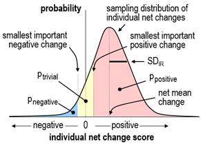
the mediator. Individual responses as a standard deviationWhen there are individual responses to an experimental treatment, the standard deviation of change scores in the experimental group is expected to be greater than that in the control group. The net mean effect of the treatment is given by the difference in the mean changes in the two groups, and the individual responses to the treatment can be summarized by a standard deviation representing the extent to which the net effect of the treatment differs typically between individuals. This standard deviation (SDIR) is not simply the difference in the standard deviations of the change scores; instead, the standard deviations have to be squared to give variances, then SDIR is given by the square root of the difference in the variances: SDIR = Ö(SDE2–SDC2), where SDE and SDC are the standard deviations of the change scores in the experimental and control groups. This formula is easily derived from statistical first principles on the reasonable assumption that the individual responses are random numbers independent of the random numbers representing error of measurement. It is also assumed that the error of measurement is the same in the two groups; if the error could differ, for example through habituation in the experimental group being different from that in the control, an extra post measurement is needed to derive SDIR, as explained in the accompanying article on SAS programs for individual responses (Hopkins, 2018a). When the design
consists only of an experimental group with pre- and post-tests, the standard
deviation of change scores in the control group (SDC) in the above formula can be replaced by an estimate from a
published reliability study with similar subjects, measurement protocol and
time between tests. The estimate (or guestimate,
if the reliability studies all have much shorter time between tests) is given
by the standard error of measurement (the typical error) multiplied by Ö2. The estimate of SDIR provides the simplest approach to evaluating the magnitude of individual responses. Magnitude thresholds for a standard deviation are half those for a difference in means (Smith and Hopkins, 2011); consideration of the proportions of positive, trivial, and negative responders for different values of SDIR provides evidence that these thresholds apply to SDIR (Hopkins, 2018b). The uncertainty in the estimate should be taken into account by interpreting the magnitude of the upper and lower confidence limits. For standard deviations and non-clinical effects, the default level of confidence is 90%. If the upper and lower confidence limits are substantial in a positive and negative sense, the SDIR has unacceptable uncertainty and is declared unclear. Estimation of the confidence limits for SDIR presents a theoretical challenge. The SDIR is estimated first as a difference in variances, and it is inevitable that the difference is negative in some samples, owing to sampling variation in the standard deviations of change scores. It may also happen that the population standard deviation of change scores in the experimental group is less than that in the control group, owing to the treatment somehow tending to bring all subjects up or down to similar post-test scores–an "homogenizing" effect that is the opposite of individual responses. It follows that estimation of SDIR and its confidence limits must allow for negative values of SDIR2, and an assumption must be made about the sampling distribution of SDIR2, if its confidence limits are to be derived analytically. When a mixed model is used to estimate SDIR2 in the Statistical Analysis System, it is estimated as a variance, and the assumption is "asymptotic normality"; that is, SDIR2 is assumed to have a normal distribution, including negative values, when the sample size is sufficiently large. This assumption follows from the Central Limit Theorem, if we assume that an individual response is due to the summation of trivial contributions of many genetic and environmental factors interacting with the treatment. Congruence of confidence limits based on this assumption and those derived by bootstrapping, detailed below, show that sample sizes of ~40 in each group are "sufficiently large". Some factors, such as gender, may produce substantial discrete individual responses, in which case the distribution of individual responses will be decidedly non-normal, but appropriate inclusion of gender in the analysis will restore normality to the distribution. The dependent variable may also need log-transformation to achieve normality of SDIR2 and uniformity of error and effects in the analysis. Since the square root of a negative number is imaginary, negative values of SDIR2 or its confidence limits result in imaginary values for SDIR. I recommend presenting negative variance as a negative standard deviation, by changing the sign before taking the square root, with the understanding that the negative values represent the extent to which there is more variation in the change scores in the control group than in the experimental group. Negative values for the confidence limits also allow meaningful assessment of the uncertainty in the magnitude of SDIR. Individual responses as proportions of respondersThe traditional approach to analysis of individual responses is to calculate proportions of positive responders directly from the individual change scores, by assuming that any positive change score or any change score greater than some threshold represents a positive response; similarly, proportions of negative responders are given by the proportions of negative change scores or scores more negative than some negative threshold, and proportions of trivial responders are given by change scores falling between the positive and negative thresholds. The threshold chosen in the past has been either the standard deviation representing the error of measurement or some multiple of it, such as 1.5 or 2.0 (e.g., Bouchard et al., 2012). The rationale for this approach is that sufficiently large positive or negative changes are unlikely to be due simply to error of measurement and can therefore be considered "real" changes. Unfortunately, even such real changes are not necessarily substantial individual responses. For example, if an individual has changed by 2.5 errors of measurement, and the smallest important change is equivalent to 3.5 errors of measurement (implying the measure is very reliable or precise), then this real change would be better characterized as a trivial individual response rather than a positive individual response. Thus, estimation of the proportions of responders from individual change scores requires not only the error of measurement to be taken into account but also the smallest important change, and the calculation has to be based on estimates of each individual's probabilities of being a positive, trivial, and negative responder. I will consider later how to calculate such probabilities. Meantime there is a more direct approach to calculating proportions of responders from the SDIR and the net mean change, as follows… If the true value of SDIR is zero, then every individual is either a positive responder, a negative responder, or a trivial responder, depending on whether the true net mean change is greater than the smallest important positive change, less than the smallest important negative change, or somewhere in between. If SDIR is greater than zero, and the distribution of individual responses is normal, it is a straightforward matter to calculate the proportions of positive, trivial and negative responders from areas under the normal distribution, as shown in Figure 1.
Again, the distribution is likely to be normal, but there are two problems: how do we calculate the proportions if SDIR is negative, and how do we calculate confidence limits for the true proportions? I have taken the following approach to solving these problems. If the SDIR is positive, we calculate the proportions in the manner shown in Figure 1, using the sample net mean change and SDIR. If SDIR approaches zero, one of the three proportions of responders will approach 100% (for example trivial responders, if the net mean change is trivial), while the other two proportions (of positive and negative responders) will approach 0%. Imagine now that the SDIR passes through zero to some small negative value. To represent the fact that the data now display the opposite of individual responses, I allow the proportions to exceed 100% (for trivial responders, in this example) or fall below 0% (for positive and negative responders). These impossible proportions are calculated by allowing SDIR to represent individual responses in the control group, by estimating proportions of responders in the usual way, then by assigning the proportions to the experimental group with appropriate changes in value (>100%) or sign (<0%). The confidence limits for the true proportions are then estimated by resampling (bootstrapping) from the original sample at least 3000 times, and for each of the 3000 samples calculating the proportions of responders exactly as for the original sample. The appropriate percentiles of the proportions in the 3000 bootstrapped samples provide the confidence limits for the true proportions (e.g., 5th and 95th percentiles for 90% confidence limits). The medians (50th percentile) of the proportions in the bootstrapped samples should also be, on average, the true proportions. In simulations to check on the accuracy of this approach (Hopkins, 2018a), I would need to perform several thousand trials each with the same chosen means and standard deviations for the true values of the various parameters, then determine how often the confidence intervals for the proportions of responders include the true proportions. Limitations on computer memory and processor speed have thus far limited my simulations to 20 trials and sample sizes of up to 80 in each group. The coverage of 90% confidence intervals is consistent with their being accurate in this limited number of trials for a range of realistic values of the mean response and SDIR (including both zero) for sample sizes of 40 or more in each group. In view of the complexity of the analysis, I do not recommend bootstrapping to compute accurate confidence limits for the proportions of individual responders. Instead, the sample estimates of the mean and SDIR along with a value for the smallest important mean change can be combined in a spreadsheet to estimate proportions of responders in the sample. The sensitivity of the proportions to uncertainty in SDIR can then be investigated by repeating the calculation with the upper and lower confidence limits of SDIR. A spreadsheet is available for this purpose via the in-brief item on sample size for individual responses (Hopkins, 2018b). The resulting confidence limits for the proportions are underestimates, because they do not account for uncertainty in the mean change, and because any negative SDIR is set to zero. Individual responses as individual probabilities of respondersIt is a relatively simple matter to evaluate the probabilities of true values of each change score in isolation: the standard error of the change score is Ö2 times the error of measurement, and with the assumption that the sampling distribution of the change score is normal, the probabilities that the real change is substantially positive, trivial and substantially negative are given once again by areas under a sampling distribution similar to Figure 1. Averages of these probabilities across all the individuals in the experimental group should then give the proportions of positive, negative, and trivial responders. Unfortunately, consideration of the proportions of responders when the true value of SDIR is zero or negative shows that this reasoning cannot be correct: the true proportions of positive, trivial and negative responders are 0% or 100%, depending on the true value of the net mean change, yet the mean values of the sample probabilities will always fall between 0% and 100%. The discrepancy arises from the fact that the individual probabilities arise partly from error of measurement, and the remaining contribution from the treatment itself has to be assessed by taking into account the changes in all the other subjects. Individual probabilities of being a responder will be unbiased only when a method can be found to allow an individual's probabilities to be <0% or >100%, when SDIR is negative. Confidence limits for each individual's probabilities could then be found by bootstrapping. In the absence of such a method, I set the probabilities in my simulations to 0% or 100%, whenever SDIR is negative in the original and bootstrapped samples. As expected, the mean proportions of responders in simulations deviate substantially from the population values when the uncertainty in SDIR allows for sample values of SDIR to be substantially negative (i.e., when the lower confidence limit of SDIR is substantial, which occurs with small sample sizes and small or negative population values of SDIR). With such data, the estimates of each individual's probabilities of being a responder cannot be trusted, so I do not recommend this approach. Statistical models for simple designsSeparate linear regressions of change scores in the control and experimental groups followed by a comparison of the effects with the unpaired t statistic provides a robust approach to estimating the mean treatment effect and the effects of modifiers and mediators. The magnitude of SDIR and its confidence limits can be derived from the standard deviations of the change scores. This approach has been realized in a spreadsheet, which also allows prediction of the mean response of individuals with chosen values of the baseline and another characteristic (Hopkins, 2017). If the analysis is performed with a mixed model, a random effect that specifies extra variance in the experimental group additional to the residual (error) variance is specified by interacting the identity of the subjects with a dummy variable having a value of 1 in the experimental group and 0 in the control group. The variance of this random effect is SDIR2, and its "solution" (the individual values that make up SDIR) is each subject's individual response additional to the net mean change. The procedure used for the analysis should allow for negative variance for the random effects, which currently excludes the open-source "R" package. The Statistical Package for the Social Sciences (SPSS) does not allow negative variance, but unlike R, it provides a standard error and a p value for the variances, either of which can be used to calculate confidence limits with the assumption of normality. (If the observed variance is negative, SPSS shows it as zero and issues an error. Rerun the analysis with the dummy variable indicating extra variance in the control group, then change the signs on the resulting SDIR and its confidence limits.) Programs for running the analysis with the procedure for mixed modeling (Proc Mixed) in the Statistical Analysis System (SAS) are available (Hopkins, 2018a). These programs will run in SAS University Edition, the free version of SAS Studio. Instructions on installing and using SAS Studio for mixed modeling are also available (Hopkins, 2016). The fixed effects in the mixed model for change scores are the usual additive terms that would be used in an analysis of variance or covariance: a nominal variable representing the control and experimental groups (which provides the mean change in each group and the net mean change, the difference in the changes), and the interaction of this variable with any subject characteristics that could be modifiers of the treatment effect. Modifiers can be nominal (e.g., gender) or numeric (e.g., pre-test fitness). If a numeric modifier has a suspected non-linear effect, it can be modeled as a quadratic or higher-order polynomial, or it can be recoded into subgroups and included as a nominal modifier. An exception is the pre-test score of the dependent variable, which should be included almost invariably as a simple linear numeric modifier. As such, this variable explains some of the variance in change scores arising from regression to the mean, whereby values of noisy measures that deviate from the mean are on average closer to the mean on re-test. Inclusion of the pre-test therefore reduces the residual error and improves the estimates of all effects in the model. For more on regression to the mean in controlled trials, see Hopkins (2006b). The effects of modifiers are evaluated as the difference in the effect between the groups defined by a nominal characteristic and the difference in the effect of two between-subject standard deviations of a linear numeric characteristic. To the extent that a modifying effect is substantial, SDIR will reduce in magnitude when the characteristic is included in the model. For a thorough analysis, interactions of subject characteristics should also be considered, and the random effects in the model should specify different individual responses and different residual errors for each subgroup defined by a nominal characteristic. If such analyses seem too daunting, I recommend separate analyses for each subgroup, which are equivalent to a single analysis with all other characteristics interacted with the characteristic and with different SDIR and residual errors for each level of the characteristic. Effects, SDIR and residual errors can then be compared and averaged with a spreadsheet (Hopkins, 2006c). In simple crossovers or pre-post trials without a control group, the modifying effect of the baseline value of the dependent variable includes a negative contribution arising from regression to the mean. This effect is automatically adjusted away when there is a control group (in controlled trials) or an additional control treatment (in crossovers). In their absence, the adjustment can be performed with data from a reliability study with subjects and time between treatments or trials similar to those in the crossover or pre-post trial. From first statistical principles, the slope between change scores and baseline score is given by -(1–r) or -e2/SD2, where r and e are the retest correlation coefficient and error of measurement, and SD is the standard deviation of the baseline scores. It is better to use the second of these two formulae, with e calculated or guestimated from the reliability study. The adjusted effect of 2SD of baseline is obtained by adding 2SDe2/SD2 = 2e2/SD to the effect. (I was unable to find a citable reference for this simple formula, so I checked it with an Excel simulation. The spreadsheet also gives a formula to adjust single change scores.) Potential mediators can also be included as fixed effects, usually as simple linear effects of change scores either interacted with the treatment effect (if you suspect mediation is not present in the control group or treatment) or without interaction (if you expect the same mediating effect–the same slope–in both groups or treatments). The effect of a mediator can be evaluated as that of two standard deviations of change scores, but more important is the reduction in the mean treatment effect when the mediator is included, and the effect of the mean change in the mediator itself; these add together to give the effect of the treatment without the mediator in the model. Individual responses will also reduce in magnitude when an effective mediator is included in the model. Statistical models for complex designsData from designs in which there is more than one experimental group (e.g., two types of training) or control group (e.g., a placebo intervention and a wait-list control) can be analyzed in pairwise fashion using the same model as detailed above, or the group effect in a single mixed model can be specified with more than two levels. A separate dummy variable interacted with the subject identity is required in the single mixed model to estimate individual responses in each experimental group. In designs where there is a short-term repeat of the post-test to account for any difference in post-test error between the control and experimental groups, analysis of the two change scores from the pre-test with a mixed model allows for specification and estimation of separate random effects for the individual responses and the errors in each group. If more than one pre-test is performed to improve precision of estimation of the individual responses, it is best to average each individual's pre-test scores so that there are still only two change scores for each individual. It is also possible to analyze original scores rather than change scores, but it is more difficult to specify the fixed and random effects, especially the modifying effect of the pre-test scores and the effects of mediators. I strongly advise use of change scores in all analyses of individual responses. With two or more post-tests separated by sufficient time for the mean response and individual responses to change between post-tests, changes in the mean are easily estimated with the appropriate fixed effect, but estimation of the individual responses in each of the post-tests is more challenging. The individual responses are not independent, because a responder in the first post-test will tend to be a responder in the second post-test. This scenario can be taken into account by using a dummy variable to specify a random effect for individual responses in each post-test, and by invoking the so-called "unstructured" variance-covariance matrix for these two random effects. The resulting variances provide the estimates of individual responses in each post-test, and the covariance provides the consistent or sustained individual responses. It is also possible to specify separate dummy variables for one-time-only individual responses in the two post-tests and a third dummy to specify the sustained individual responses with the independent "variance components" structure; this approach provides confidence limits for the one-time-only individual responses. The error of measurement in the above design may change between the two post-tests, but it is assumed the same change occurs in the control and experimental groups. With the more realistic assumption that the change in error differs between groups, short-term repeats of the post-tests are required to account for and estimate the differences in errors. A random effect specifies the changes between the pre-test and the two main post-tests that happen equally in both groups, and the same random-effect dummy variables as in the previous model are used to specify the individual responses due to the treatment. Separate measurement errors are specified as four separate residuals for the groups and the two main time points. See this article for details of the realization of this model and the other models in SAS (Hopkins, 2018a). I am skeptical about the practical relevance of models based on individual differences in linear time-dependent increases in fitness with repeated testing during a period of training, as described in the consensus document from the symposium on individual fitness responses (in preparation). Adaptation to a constant dose of training is non-linear: there is a rapid increase in fitness reaching a plateau after 4-8 weeks. With the usual progressive increases in dose, fitness will increase, but there is no way one can ever assume a linear increase in the fitness response. The analyst is stuck with assessing fitness at several time points and assessing changes between points in a pairwise fashion–hence the models above with two post-tests. Acknowledgements: I thank Claude Bouchard for the opportunity to participate in the symposium on individual responses and the Pennington Biomedical Research Center for funding travel and accommodation to Baton Rouge. Thanks also to Alan Batterham for reviewing the manuscript and providing numerous important suggestions for improvement. ReferencesHiggins JPT, Green S (2011). Cochrane Handbook for Systematic Reviews of Interventions Version 5.1.0 [updated March 2011]. Cochrane Collaboration. www.cochrane-handbook.org. Accessed 15 Jan 2016. Hopkins WG (2006a). Estimating sample size for magnitude-based inferences. Sportscience 10, 63-70 Hopkins WG (2015). Individual responses made easy. Journal of Applied Physiology 118, 1444-1446 Hopkins WG (2016). SAS (and R) for mixed models. Sportscience 20, iii Hopkins WG (2018b). Sample size for individual responses. Sportscience 22, i-ii Mastrandrea MD, Field CB, Stocker TF, Edenhofer O, Ebi KL, Frame DJ, Held H, Kriegler E, Mach KJ, Matschoss PR, Plattner G-K, Yohe GW, Zwiers FW (2010). Guidance Note for Lead Authors of the IPCC Fifth Assessment Report on Consistent Treatment of Uncertainties. Intergovernmental Panel on Climate Change (IPCC): https://www.ipcc.ch/pdf/supporting-material/uncertainty-guidance-note.pdf Published August 2018 |